This is part of the series behind the scenes of RP2040 Doom:
- Introduction
- Rendering And Display Composition
- Making It All Fit In Flash <- this part
- Making It Run Fast And Fit in RAM
- Music And Sound
- Network Games
- Development Overview
See here for some nice videos of RP2040 Doom in action. The code is here.
Compression Introduction
As mentioned in the main introduction, everything in the WAD (level data, sound effects, music, graphics and textures) must be compressed in order to fit in our tiny amount of flash space. The compression methods used have to allow for random-access to all data, as there isn’t any spare RAM to decompress even just one level’s worth of data into RAM at runtime.
The WAD may contain tens of thousands of certain types of structures or fields, so every single byte in such structures or fields had to be agonized over, as they may each cost 10s of kilobytes or more overall.
The WAD is converted by the new tool whd_gen (WHD stands for “Where’s Half the Data?”) which can produce a .WHD
file or a .WXD file, the latter being smaller but with more restrictions on the input WAD.
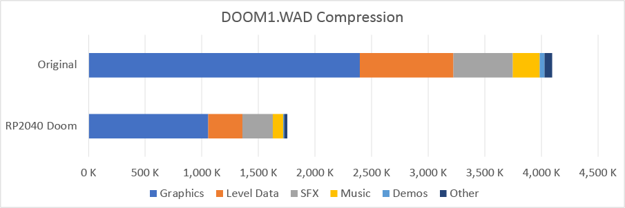
The DOOM1.WAD is 4098K big. DOOM1.WXD is 1758K, i.e. a healthy 57% compression. This compression is
basically lossless except for the sound effects which are ADPCM encoded.
In addition to squashing the WAD, I needed to take a hatchet to a lot of the read only data and tables used by the Doom Engine, and of course, minimize the size of the actual code itself. The resulting RP2040 Doom executable, with code and static data, all fit into 256K of the flash.
This leaves 34K (woot) on a Raspberry Pi Pico, with its 2M flash, to persist up to six saved games. Since vanilla Doom saved games range from about 10K to 60K+, the saved games also need to be heavily compressed!!
This whole section gets quite involved in places, so no one will be offended if you just skim through to whichever ones you think are more interesting!
General Compression Methods
The following general lossless methodologies are used to compress data:
-
Smaller data types: If a 16-bit integer will do, use that instead of a 32-bit integer.
-
Packed C bit-fields in structures: Occasionally this can be used to shrink a structure whilst keeping the structure properly aligned (e.g. using two 12-bit values to fit in 3 bytes).
-
Compressed structures: Whilst changing data types can minimize the size of structure, it necessarily applies to all instances of a particular structure. However, I noticed that often some individual fields of a structure may be:
- Frequently, but not always, zero.
- Frequently, but not always, 1 byte not 2 bytes.
- In some way predictable based on other structure fields, or external information (e.g. the structure’s index within an array).
I can take advantage of such probabilistic information to devise a menu of different encodings for the structure. Therefore, a set of bit flags are included in the structure that indicate which of the various possible encodings are in play for that instance, dictating the particular size of the structure for that instance. In this way the expected (average) size of the structure is reduced.
Macros or functions are used at runtime to decode structure fields, and use non type-safe
uint8_t *pointers to refer to instances. Integer indexes into arrays of such structures can be replaced by integer byte offsets from the start of the array, and arrays of structures can still be iterated in order, since the size of each element can be determined. -
Variable byte-count integers Sometimes, when their sizes are often expected to be small, integers are encoded as a variable number of bytes, LSB first, with 7 significant bits and a flag in each byte. The flag indicates whether another byte of significant bits follows.
For signed integers the values are “zigged” into unsigned values by renumbering 0,-1, 1, -2, 2, -3 to 0, 1, 2, 3, 4, 5 etc. These types of variable-number-of-bytes integers are generally used in otherwise byte-centric streams of data.
-
Variable bit-lengths: For unstructured data, the data stored is just a series of values. It is much more efficient to encode these values as arbitrary bit lengths, rather than in multiples of bytes.
The data is therefore encoded as bit-streams with the bit-length of each value dependent on the value type and its context. Whilst 5 bits may always be used for one certain value type, it is often possible to use additional contextual information to optimize these bit lengths further.
As an example, if you are encoding the run-length of opaque pixels in a vertical strip of a graphic, the number of bits needed to encode the run-length is certainly no more than required to store the remaining length of that strip to the bottom of the graphic from where you are.
-
Huffman Coding: Sometimes it is not just the context of the value that best determines the bit-length used to encode it, but also its probability. When one value (“symbol”) is more likely than others, a sequence of symbols can be compressed by using shorter bit-lengths for common symbols, and longer bit-lengths for rare symbols.
In Huffman Coding, symbols are assigned “codes” (a unique string of bits) where no “code” is the prefix of another.
More on the RP2040 Doom Huffman Coding
Huffman coding converts a string of input symbols into a series of variable bit length prefix codes. What the symbols represent is entirely up to the use case.
Many compression methods (e.g. Zip) use an input symbol alphabet which includes raw byte values, but also
symbols for references to previous sequences of bytes in the stream. (e.g. one symbol might represent the byte 0x41
and another
might represent
“the
sequence of 7
bytes
just decoded 32 bytes ago”). This is called (LZ77) dictionary compression and is very efficient when you expect many
sequences of bytes to repeat.
Such dictionary compression methods are suited to long streams of data where you can keep significant decoded history data to copy byte sequences from (Zip keeps 32K by default). You cannot decode just a short sequence in the middle, without decoding everything before it. RP2040 Doom needs to be able to encode and decode really short (10s of bytes) sequences of data, so the dictionary method is a bad choice.
Like Zip however, an optimal set of Huffman Codes are generated based off the probability distribution of the input symbols measured at compression time. These codes might be common to an entire graphic, but can still be used to decode just one column of that graphic independent of the rest.
The decoder must know the Huffman Codes that were used by the encoder, so the codes or the probability distribution must be stored too. Again like Zip, the code lengths for each symbol in the input alphabet are what is stored, which is sufficient information for the decoder to regenerate the Huffman Codes.
In the simplest case, the input symbols universe might just be the 256
possible 8-bit values representing palette indexes used in a graphic. Some possible symbols are never used
in a particular entity, so are assigned a code length of 0. The remaining one are assigned codes according to
their frequency (e.g. if a graphic only used palette
indexes A, B, and C, and A was the most common, then they would be assigned bit lengths 1, 2 and 2. From this
information both the encoder and decoder can derive a common set of codes (e.g. A = 0, B = 10, C = 11).
In the above example only 3 out of 256 possible symbols are used and thus have codes, and this sort of sparseness is common. This known sparseness, along with additional knowledge RP2040 Doom has about the input symbol alphabets, can be used to devise ultra-compact packed representations of the used symbols and bit-lengths according to entity type. This is slightly different from Zip which has no a-priori information about the likely distribution of the input data bytes themselves, and thus uses some extra meta-levels of Huffman Codes to describe the symbols’ code lengths compactly.
Much of the hard work here of course is picking a set of symbols to encode. Whilst raw input bytes are used as a possible symbol alphabet in the examples above, compressing these directly does not generally yield the amount of compression required, so higher-level symbols must often be fashioned, with much more differentiating probability distributions.
Compressing the WAD
The WAD in Doom is made up of named “lumps” which are individual assets (graphics, sounds, level elements, etc.) that are combined into a coherent whole by the game engine. The vanilla Doom engine supports combining WAD files together at runtime allowing one WAD to override lumps in another WAD by name.
Since RP2040 Doom requires a single read-only WHD (our version of WAD) image in flash, any ability to patch the WAD at runtime is removed. If the user wants to alter base WADs they can do so with existing host side tools before generating the WHD. When the WHD is generated, therefore, 8 character lump names can be replaced with 2 byte lump numbers saving some space. Not all names can be removed as some are referenced explicitly by the Doom code.
The remainder of the space-saving comes from actually compressing the lumps within the WAD.
You can refer to Doom Wiki - WAD section to get a bit more detail about the types of lumps mentioned below.
This section uses the shareware DOOM1.WAD as an example, as this is the target needed to be fit in the 2M flash on
the Raspberry Pi Pico.
It turns out that for DOOM1.WAD pretty much everything that could reasonably be compressed, needed to be in order
to get
everything to fit in 2M.
The ( %) in the headings are the savings for each item in DOOM1.WAD.
Graphics Compression (56%)
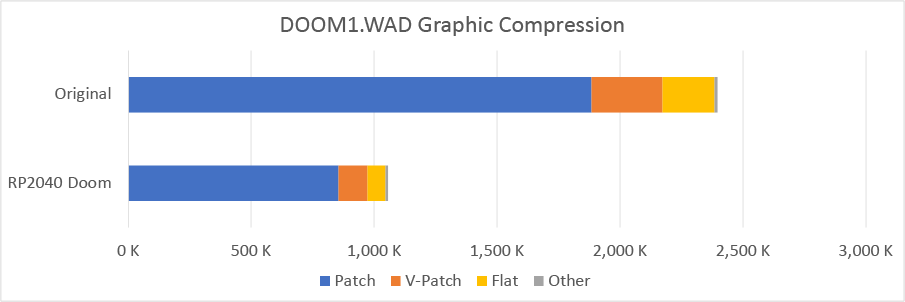
Patches (54%)
A patch in Doom is a graphic made of vertical runs (posts) of pixels. These are used for sprites, wall textures, menu graphics etc. (basically any graphical element except for floors and ceilings). Patches are stored vertically because all sprites and wall textures are rendered as vertical strips by the Doom engine. This rendering order is convenient as all such vertical strips have the same Z value, so no perspective correction or light level adjustment is needed down the strip, and so the rendering loop can be very fast.
In RP2040 Doom the patches that are not used for 3D rendering (i.e. not game sprites and parts of wall textures) are treated as a separate category called (by me) “V-Patches” and handled completely differently. The compression of these V-patches is described later.
RP2040 Doom takes the size of regular patches in DOOM1.WAD from 1880K to 851K.
This is what a patch looks like in vanilla Doom.
Patch:
Field      Type       Size       Offset      Description
width      uint16_t   2          0           Width of graphic
height     uint16_t   2          2           Height of graphic
leftoffset int16_t    2          4           Offset in pixels to the left of the origin
topoffset  int16_t    2          6           Offset in pixels below the origin
columnofs  uint32_t[] 4 * width  8           Array of column offsets relative to the beginning of the patch header

Each column is an array of post_t, of indeterminate length, terminated by a byte with value 0xFF (255).
Field      Type       Size       Offset      Description
topdelta   uint8_t    1          0           The y offset of this post in this patch. If 0xFF, then end-of-column
length     uint8_t    1          1           Length of data in this post
unused     uint8_t    1          2           Unused padding byte; prevents error on column underflow.
data       uint8_t[]  length     3           Array of pixels in this post; each data pixel is a palette index
unused     uint8_t    1          3 + length  Unused padding byte; prevents error on column overflow
Note: there are 44577 patch columns and 61731 posts in DOOM1.WAD
The following explains how RP2040 Doom deals with the the regular patches:
-
The pixel data is separated from the “patch metadata” which describes the individual pixel run lengths.
-
A single set of symbols and code lengths is used to encode all the pixels in the patch. There are two different possible encoding schemes (way of assigning symbols) used, and the one which compresses the patch the best is chosen.
-
Data remains accessible column by column.
-
Identical columns are not encoded twice.
-
Fully opaque patches, which are quite common for patches used as wall textures, are flagged as such, and no post metadata is kept.
-
Unlike vanilla Doom, no padding bytes are stored. Each patch column is decoded into a temporary buffer at runtime before rendering, and that runtime buffer is padded with duplicate bytes at the top and bottom to achieve the same protection.
Encoding pixels
Each post within the patch is stored as a sequence of symbols according to the encoding scheme chosen.
This is either:
-
The simple version. Each symbol is just a palette index for a pixel. Compression occurs, because some pixel colors are more likely than others within the patch. Also, most patches have considerably fewer than 256 different colors, so the Huffman Codes for each pixel value even if evenly distributed, would naturally be shorter than 8 bits.
-
The more complex version, which turned out to be necessary because just performing the above compression does not save enough space, saves another 130K or so by taking advantage of the nature of the graphics and the palette used in Doom. This is described below:
Given that only 256 colors are available, and to better support the atmospheric lighting, the vanilla Doom palette is split into a bunch of color bands as shown below:
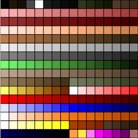
The vanilla Doom engine supports rendering any color at one of 32 different brightnesses. However, the color used for each brightness for each of the 256 colors in the palette, must itself come from the same palette. The use of color bands makes this effect much more pleasing:
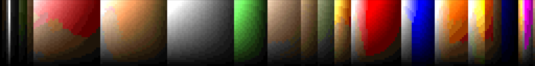
The sprites themselves were based on real world models and very often, large areas are made of the same basic color, and thus in the same color band:

Most importantly the palette is ordered such that lighter and darker versions of the same base color are at adjacent palette indexes. As you see in the boss image above, there are often smooth color variations as you move down a column in the patch, and because of the palette ordering, these color variations map to small changes in palette index from pixel to pixel.
To take advantage of this, in the second encoding scheme, an extra seven symbols are added in addition to those for the raw palette indexes, and encode a delta from the previous palette index in the column. Deltas in the range -3 to +3 were selected, as these turn out to be most beneficial (hence 7 different symbols). These new delta symbols are common as they cover a wide range of smooth color variations, and therefore tend to have shorter bit lengths than the raw colors they replace.
I tried a bunch of other - what I thought were fantastically clever - encodings, but the moral of the story seems to be that adding complexity generally adds an equal amount of encoding overhead, so. sticking with this simple strategy actually gave the best results.
Side note, and lesson learned while playing with the pixel encodings: If it seems to good to be true, it probably is! I learned my lesson early on to always decode what I had just encoded for validation before I put that space-saving in the bank. Sadly even this wasn’t even enough, and at one point I found that I had saved an amazing about of space, only to realize that I had accidentally left in some pixel pre-processing I was using to visualize possible compression techniques by looking at PNGs of the patches. These modified images compressed really well, and decoded correctly back to themselves, but of course weren’t the data I was supposed to compressing!
Encoding patch metadata
The header in RP2040 Doom is now 6 or 8 bytes:
flags      uint8_t    1                (fully-opaque, 2-byte-offsets, byte-column-offsets)
width      uint16_t   2                Width of graphic
height     uint8_t    1                Height of graphic
leftoffset int16_t    1/2              Offset in pixels to the left of the origin
topoffset  int16_t    1/2              Offset in pixels below the origin
followed by Huffman Code information for pixel decompression:
decodesz   int8_t     1                Size of decoding tables (/2) that will be needed to decode pixel data
encdoing   ?          variable         Encoding of Huffman Codes for pixel data.
and then the column offsets:
columnofs uint16_t[] 2 * (width + 1) Array of column offsets relative to the beginning of the patch header
The compressed patch data always fits easily within 65536 bytes, so 16 bits is fine for the column
data
offsets. Since all the data is encoded as bit streams, byte alignment is not required. If 16 bits is good enough to
encode
all the column data offsets as bit offsets rather than byte offsets, then the column data is packed on bit
boundaries rather than byte, thus saving on average patch_width/2 bytes per patch.
The most fun perhaps (and you may have noticed the columnofs array has grown by one) is that RP2040 Doom actually
needs to
store two sets of data per column; the pixel data and the metadata describing the post lengths. Since there are 40K+
columns, I don’t want to keep two lengths, so I sandwich the data between columnofs[x] and
columnofs[x+1]. The compressed pixel data is stored and decoded forwards from the column offset, and the compressed
metadata is
stored and decoded backwards from the next column offset. An explicit length is not stored for either piece; it is
up to the
decoder to know how much data to read (the security conscious can get back up off the floor!)
One final wrinkle, is that offsets of the form 0xffnn are reserved to indicate that the offset is not an actual
column
offset
to the data for this column, but rather that this column is an exact copy of column number n.
V-Patches (59%)
As mentioned above, these are the subset the patches that are not part of the 3D view itself, i.e. they are
graphics for the menus, status bar,
intermission screen, etc. I named this category “V-Patches” as they are traditionally rendered in
vanilla Doom by
V_DrawPatch related methods.
RP2040 Doom takes the V-Patch size in DOOM1.WAD from 286K to 117K.
If you read the section on rendering, you’ll know that these V-patches must be drawn as horizontal strips rather than vertical strips, and that a lot of them must also be drawn, very fast, every frame.
The potentially large number of different V-patches used in any one frame, and the up to 60fps rendering speed required, both preclude using the regular Huffman Code based pixel compression, so instead, fixed bit-width values are used for each pixel:
-
Depths of 4, 6 and 8-bit are supported. Generally these ranges (up to 16, 64 and 256 unique colors) are good characterizations of the sorts of graphics which are used as V-patches. On rare occasions (mostly the red menu text) the number of colors may be reduced from 17 say to 16 with little noticeable effect.
-
Usually each V-patch stores its own n-bit index->8-bit palette color mapping, but referring to a shared color-mapping is also supported. Three such color mappings in use in RP2040 Doom, one for example is used for all the previously mentioned red menu text. These shared color-mappings used are actually used for speed reasons rather than space reasons, as the palette can be pre-converted once, saving an extra lookup per pixel in the V-Patch rendering loop.
-
For each bit depth supported, up to three different encodings as needed to handle transparency:
- Fully Opaque. If a V-Patch is fully opaque, it can be marked as such avoiding the need to store any other transparency information, but more importantly, allowing it to be rendered much more quickly at runtime.
- Transparent Index. An n-bit value is stored for every pixel, but the value 0 is used to indicate transparency.
- Oppaque/Transparent Run-lengths. Lengths for each run of opaque or transparent pixels within a V-patch row are stored. n-bit pixel values are only stored for the opaque runs of pixels. This is generally more compact and faster to render than the “Transparent Index” type, except when dealing with small fiddly font glyphs.
The data for each pixel row within a V-Patch is stored in such a way that, given a data pointer to the start of the row and the V-Patch width and encoding, a row can be rendered leaving the data pointer pointing to the next row. This facilitates drawing the V-patch incrementally, line-by-line, whilst maintaining mimimal state.
Texture Data (16%)
A “texture” in doom is used to cover the vertical walls (or parts of walls) in the 3D View. Each texture is “composed” by drawing one or more patches onto a logical canvas of a certain size. The use of patches, rather than storing each texture as its very own bitmap, allows a much wider variety of textures to be created in a small mount of space. The same small selection of say “stone-like” patches can be placed next to, or over each other, creating set of larger more random diverse looking textures. Additionally, “decal” patches can be drawn on other patches to customize textures as is often done for “switches” in Doom.
Vanilla Doom creates some large runtimes structures in RAM to describe the net effect of all this compositing on each column within each texture, and indeed keeps a cache of pre-rendered columns since they are quite expensive to draw.
In RP2040 Doom, there is no space for these runtime RAM structures, so additional data is encoded in the WHD describing key facets of the texture for direct use at runtime. Fortunately this additional data, after suitable compacting measures, still ends up smaller than the original texture information.
The vanilla Doom texture information, includes basics such as width and height, along with a list of patches, and the coordinates they are drawn at.
In RP2040 Doom:
-
The basic width, height data etc. are stored compactly along with new bit flags.
-
Any texture which is made of a single patch drawn at the top left of the texture is flagged as such. It is not uncommon for a single patch to be used as a wall texture, and so no additional metadata is stored for this type of texture. Note that all textures with transparency happen to be of this type too.
-
If there is more than one patch, additional metadata is kept that is described below. This metadata contains a local palette of (up to 16) patches used within the texture to avoid referring to textures by their full 16-bit identifier.
The rendering path at runtime is much more costly for any texture column that doesn’t just consist of a single column from a single patch. Often, textures have many single patch columns even if other columns are “composite” (drawn from multiple patches). An example of such a texture with some single patch columns and some “composite” columns, would be a large patch which has a smaller patch opaque rectangular patch drawn in the center. The texture columns to the left and right of the center patch, are identical to single columns in the larger patch, and are thus called “one-patch” columns.
A very simple run length encoding is kept of alternating counts of “one-patch” vs “composite” columns across the texture. In the above example, it might be 96 “one-patch” columns from patch A, then 64 “composite”, and finally 96 “one-patch” from patch A again. This run-length metadata is used early on in the RP2040 Doom scene rendering to identity texture columns that are actually just patch columns (in this case patch A), and send them down a much faster rendering path.
Composite Columns
Another series of run-lengths across the texture is kept for runs of “composite” columns that are drawn from the same source patches in the same way. In the simple example above, all the 64 “composite” columns would be in the same run, as they have some of patch A at the top, some of the smaller patch B in the middle, and some of patch A at the bottom. The only difference from one column to the next is the x-position of the source data in patches A & B.
All columns in the run are drawn in the same way. and the metadata stored for the run is a set of drawing commands used to “compose” the column. Each simple command draws a contigous vertical strip of pixels. In the example above, 128 pixels might be drawn from local patch 0 as the background and 40 pixels from local patch 1 at y position 60 on top.
Each drawing command type is a variable number of bytes, and is comprised from the following:
- End of strips marker (1 bit): marker for the end of the strips used for this run of columns.
- Strip length (7 bits): The length (height) of the strip minus one.
- Local Patch Number (4 bits): the local patch to draw from (if any).
- Flags (4 bits):
explicit_y,memcpy,memcpy_source,memcpy_backwards - Starting y-offset (8 bits): Only present if
explict_y == 1, this is used to draw over previously drawn pixels, instead of immediately following on from the bottom of the previous command. - X/Y-offsets (8 bits each): Only present for regular (
memcpy == 0) columns, these indicate the pixel used for the top of this command in the left-most column in the run. - Source position (8 bits): Only present for
memcpy == 1, columns, indicates the source position in the texture column to copy from.
These commands are interpreted at runtime to render the column into a temporary buffer containing the composited texture column, which is then immediately used for rendering.
The command set is calculated and optimized by the whd_gen tool to minimize the number of strips and use memcpy
when possible. For example, if the same patch source column is repeated in the same texture
column, using memcpy avoids the need to decompress the same source patch multiple times when compositing the
texture column. As a further optimization, the memcpy can be done in either
direction to either
cause or prevent overwriting the source data during the copy. Overwriting the source data can be useful, as there are
frequently
textures which are
the same patch
stacked 2,
4, 8 or even 16 times on top of each other, and whd_gen is able to optimize the instructions to just draw the first
patch,
and then do a single memcpy for 15x the distance in order to draw the rest.
Finally, note the memcpy_source flag. At runtime, as an optimization, only as much of the column as is
actually visible anywhere in the frame being rendered is decoded. Often the level design has some portion
of a given texture always invisible above the ceiling or below the floor. Pixel runs that are the source of a memcpy
must be marked, so that their pixels are always drawn to the buffer, even if not visible, in case they are copied to
otherwise
visible
areas by memcpy.
The Doom Palettes (97%)
As discussed above, the Doom has a 256 color palette which is a total of 768 bytes (8-bit R,
G and B for
each
color). However,
the WAD
actually
stores 33 additional copies of the palette, tinted towards different colors, mixed with red for pain, mixed with
green for item collection etc. Assuming all
the WAD palettes can be derived exactly from the base palette using the original Doom formula, the whd_gen tool omits
all 33
remaining palettes, saving a bunch of space. There is plenty of time at runtime - at most once per frame - to
calculate the
actual tinted palette.
Level Data Compression (63%)
After the graphics, the level data itself is the remaining majority of the WAD.
In vanilla Doom, the game does not run directly off the WAD data in memory. Instead, a single level’s worth is instantiated into more efficient RAM structures at runtime. This is because the WAD was stored on disk, which wasn’t fast enough to access during gameplay, but also because they needed to be able to stitch multiple WADs together at runtime.
Whilst our WHD data stored in flash isn’t as fast as RAM, there is no spare RAM to copy the data to, so the data in flash must be used directly.
But as already stated, the data must also be compressed, so that compression must be done in such a way that RP2040 Doom can use the compressed data directly at runtime. There is certainly some runtime overhead for the decompression of compressed data at runtime, but this is actually probably amortized quite a lot by the reduction in slow flash traffic anyway.
I can moan as much as I like, but I have to make it the data small enough, and if I have to reclaim speed somewhere else, then so bet it!
This is the compression we achive for the various level data elements in DOOM1.WAD:
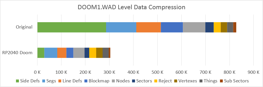
What follows is a brief(?) description of all the different types of level data lumps and how they are compressed. The italicized quotes are a brief description of the level data lump type, many of which are taken from the Doom Wiki.
All of the compression
techniques are used in WXD file used to squeeze DOOM1.WAD onto the 2M Raspberry Pi Pico, but some are currently skipped for
WHD files used when converting Ultimate Doom,
or
Doom II WADs for larger flash sizes. These larger WADs exceed some of the limits currently imposed by the WXD
format, but these WADs are less constrained in 8M than DOOM1.WAD is in 2M, so the most aggressive compression is not
needed.
Note that there is one of each type of lump per level.
LineDefs (62.58%)
“Linedefs are what make up the ‘shape’ (for lack of a better word) of a map. Every linedef is between two vertices and contains one or two sidedefs (which contain wall texture data).”
If you look at the following table you see that there is a huge correlation between many columns and the index
within the array (first column). This happens as a result of the way the level data is exported by the level editor;
note that all the WADs I have tried exhibit this behavior, but if not, it would be theoretically possible for
whd_gen to perform a reordering.
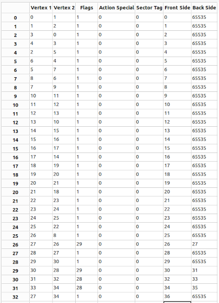
Rather than storing a 16 bit vertex index for “Vertex 1”, and “Vertex 2”, an 8-bit signed difference between the value and a “predicted” value can be stored. The predicted value is just a linear interpolation between 0 and the maximum vertex number across the range of the array.
I also noted that “Action Special” and “Sector Tag” are often (always in the subset shown) zero, and I can therefore use a variable sized struct field and a flag to say whether the value is stored.
Finally, you’ll note that “Back Side” is always either 65535 or "Front Side" + 1
(another artifact of the level export) and thus that field can actually be encoded in a single bit!
Note: when discussing predicted values, I’d said that the predicted vertex value was linear with array index.
However I cannot use array indexes to refer to “linedefs” since they are variable-sized structs, and for those,
byte-offsets are used rather than array indexes to refer to array elements. The good news is that the byte
offsets are just as reasonable a basis to use for the prediction as array
indexes; I can just predict vertex_count * lindef_byte_offset / linedefs_total_byte_size instead.
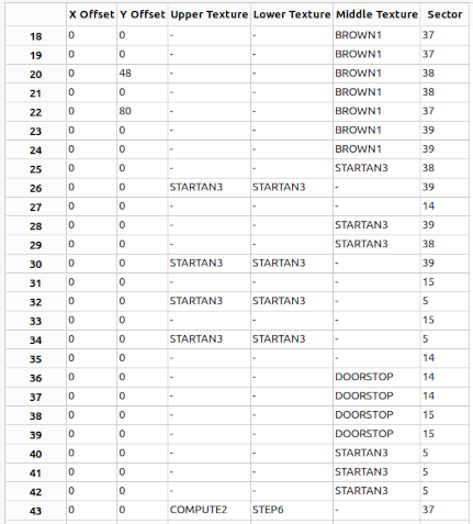
SideDefs (90%)
“A sidedef contains the wall textures for each linedef, with texture data, offsets for the textures and the number of the sector it references (this is how sectors get their ‘shape’).”
I also make “sidedefs” variable-sized structs because various fields are often zero, or can often be stored in one byte not two.
Additionally though, each “sidedef” references three textures, a “top/upper”, a “middle” and a “bottom/lower”. Space has already been saved by using 16 bit lump numbers rather than names for each of these textures, however with 30000+ “sidedefs”, storing 6 bytes per “sidedef”, the size still really adds up.
Fortunately, once again, there is a lot of correlation within the texture values for an individual “sidedef”:
There are actually only 16 possible patterns of texture values; the 8 obvious ones where each of the 3 textures places is either set to its own unique value or is blank, and 8 additional ones where the same texture name appears in more than one place. Fortunately for us, the majority of patterns only require a single texture name, as seen in all but the last “sidedef” below. Therefore, I just store the 4-bit pattern selector value, and then append as many texture number(s) as the pattern requires.
Segs (57%)
“Segs are the portions of linedefs making up the border of a subector.”
RP2040 Doom saves about 50% by using variable sized structures and some custom fixed bit-width fields.
SSectors (Sub Sectors) (50%)
“Sub sectors represent a convex region within a sector. They are a list of any segments which lie along their boundary.”
This is how the vanilla Doom WAD stores a sub sector:
typedef PACKED_STRUCT (
{
  short		numsegs;
  // Index of first one, segs are stored sequentially.
  short		firstseg;
}) mapsubsector
RP2040 Doom saves exactly 50% because we can avoid the numsegs field. The segments are already stored in sub sector
order, so the number of segments in sub sector n is actually just subsector[n+1].firstseg - subsector[n].firsteg
Nodes (50%)
“The nodes lump constitutes a binary space partition of the level. It is a binary tree that sorts all the subsectors into the correct order for drawing in the 3D view. Each node entry has a partition line associated with it that divides the area that the node represents into a left child area and a right child area. Each child may be either another node entry (a subnode), or a subsector on the map.”
Here is some node data from a level in DOOM1.WAD:
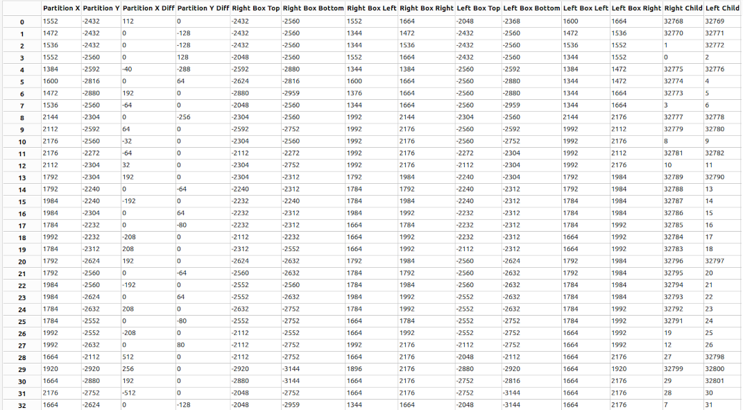
There seems to be a bunch of data here, but it can be hacked away at, fairly well.
Firstly the last 2 fields (Right Child/Left Child) can be reasonably well predicted based on node index similarly to
previous types of level data, after the top 0x8000 bit which indicates whether this is a sub sector
leaf
index or a child node index for each has been masked off. RP2040 Doom stores these two bit flags, and the deltas from
the
predicted
values for
both left
and right in 16 bits total, although different encodings are used depending on the sub sector/leaf status
of the children.
Additionally, there is some slightly wasteful information stored for each node. There are 8 16-bit values used to describe the bounding box for each child of the node. These bounding boxes are intersected with the view frustrum at runtime to determine if the child node (and thus any of its subtree) is possibly visible on screen.
I have said two important things in that sentence:
- That the children’s bounding boxes are necessarily contained within the parent’s bounding boxes.
- That this is just an optimization; it doesn’t matter if our bounding boxes are slightly too large.
Therefore, instead of storing 4 16-bit values per child, 4 4-bit values are stored that describe the bounding box of the child on a 16x16 grid laid over the bounding box of the parent. I did calculate the over-coverage at one point, and I think it is pretty miniscule, though I don’t recall the number now.
Blockmap (68%)
“The blockmap is a data structure used for collision detection. The blockmap is simply a grid of “blocks”’ each 128×128 units. Every block contains zero or more linedefs indicating which linedefs intersect with that block.”
Vanilla Doom stores 2 bytes per block which is an index into a single array of the block map’s “linedef” numbers
where that block’s list of “linedef” numbers are stored. That list starts with a 0x0000 value, and the list
is terminated with an 0xffff. The “linedefs” numbers for the block are contained between those two markers.
This means that even an empty block that is crossed by no-lines takes 6 bytes, and as you can imagine if you imagine a Doom level drawn on a grid, such empty blocks/space are not uncommon.
The RP2040 Doom storage of the “blockmap” is perhaps the most agressive/complicated of the level data:
-
For each row (same y-position) in the “blockmap”, a 16-bit base index is stored, along with a bitmap with 1-bit for each block x-position indicating whether that block is non-empty.
-
A 16-bit value for each non-empty block in the row is stored sequentially starting at the 16-bit base index for the row that was mentioned above. This is 16-bit value is located quickly at runtime by counting set bits in the bitmap from the start of the row.
-
A value with bit pattern
0b ffff nnnn nnnn nnnnindicates a block with a single “linedef” numbern. -
A value with Bit pattern
0b cccc ccxx xxxx xxxxindicates a block withc+1“linedefs”, which startxbytes after the end of the row’s block-population bitmap. -
Each “linedef” is stored as a variable-byte-count integer.
Sectors (46%)
“A sector is an area referenced by sidedefs on the linedefs. It stores the floor and ceiling textures (flats), along , floor and ceiling height, lighting level and other flags for a region within the map.”
Currently, lump names are just converted to indexes. I could save an extra byte here easily enough, but then it would blow the 16-bit struct alignment for very little saving, as there really aren’t that many sectors.
Things (0%)
“Things represent players, monsters, pick-ups, and projectiles. They also represent obstacles, certain decorations, player start positions and teleport landing sites. While some, such as projectiles and special effects, can only be created during play, most things can be placed in a map, and are created when the level is loaded. The Things lump stores these items.”
RP2040 Doom does not currently compress this lump type. Vanilla Doom stores 5 fields in 10 bytes, and this could be shrunk to 8 by converting the angle/flags field to one byte each, however this only saves about 5K over all.
Vertexes (0%)
“Vertices are nothing more than coordinates on the map. Linedefs and segs reference vertices for their start-point and end-point. The VERTEXES lump is just of a raw sequence of x, y coordinates as pairs of 16-bit signed integers.”
The full 16 bits of the coordinates are needed, and the vertexes are not stored in any predictable order, so this lump type is not compressed.
Reject (0%)
“The Reject lump is used to speed up line of sight calculations. For every sector there is a bit stored for every other sector indicating whether any of that other sector is visible from the first sector.”
Even though this lump type is fairly sparse, it is hard to compress it and maintain random access. Therefore, this lump type is not currently compressed, although if really needed to, I would probably have tried a Bloom Filter.
Sound Effect Compression (49% lossy)
In vanilla doom these are stored as 8-bits mono samples. RP2040 Doom uses ADPCM to lossily compress them to 4-bit samples along with extra metadata for groups of samples.
Music Compression (62%)
RP2040 Doom takes the size of the MUS music (A Doom format similar to single track MIDI) from
240K to 91K. Currently, only the MUS format is supported, as this the only format used in the regular Doom WADs, even
though Chocolate Doom supports full MIDI too. Previously I had a technical reason not to support multi-track
music, however this limitation was tied to the
previous Zip-like compression I tried, and so no longer really applies.
A Doom MUS file is made up of a series of events; each event starts with a first byte:
0b LEEE CCCC - where EEE is one of 8 event major event types and CCCC is the 4-bit channel number.
Each event byte is followed by a variable number of bytes depending on the event type, and the data for the current
event is immediately followed by the first byte of the next event, unless the current event has the L (Last) bit in
its lead byte set. In this case, this is the last event in a group of events for the same time code, and
is followed by a time delta encoded as a variable-byte-length integer.
There are a 6 major event types used in the MUS format; the highlighted value in {} is the event data payload if
any:
- Release note
{note number}. Release the specified note on this channel. - Play note
{note number}{note volume}. Play the specified note at the special volume on the specified channel. The note volume can be omitted, in which case the previous volume used on this channel is used. - Pitch wheel
{pitch change}. Bend the notes on the specified channel up or down in pitch. - Change controller
{controller number} {value}. Affect various attributes of the specified channel including pan position, volume, vibrato, reverb, in addition to instrument selection, and a few others. - System event. Other non-channel related events (the system event type is stored in the channel slot).
- End of track. Just that!
The entire crux of the compression is to find a sensible set of symbols to encode all the data from the MUS as compactly as possible using Huffman Coding. The encoding ends up using a good number of different probability distributions for data based on the context within which it is found.
First the MUS events are trans-coded into eight major event types of my own, incorporating the commonly used ones as first-rate citizens:
typedef enum musx_event_type
   system_event = 0x0,
   score_end = 0x1,
   release_key = 0x2,
   press_key = 0x3,
   change_controller = 0x4,
   delta_pitch = 0x5,
   delta_volume = 0x6,
   delta_vibrato = 0x7
};
Event Group Encoding
Rather than the original one-byte header, all the events for a single time code are represent as the following single sequence of symbols:
{group_length_symbol} {channel&event) ... event payload ... {channel&event) ... event payload ... {time
delta}
The first symbol is just the number of events that follow for the same time code. This length symbol (with its own Huffman Code distribution) gives better compression on average than one bit per event!
Channel & Event are combined into a single symbol because different events are more or less likely, indeed some event types are not present, on some channels versus others. Additionally, not all channels are used in a given song, and therefore do not need codes. Every used channel/event pair has its symbol with its own code length.
Individual Event Encoding
The data for each event type is then itself encoded using a custom set of per event type symbols. You’ll notice
above
that there are delta_pitch, delta_volume, delta_vibrato whereas the original MUS actually uses absolute values.
Generally these values change by small increments throughout the song, and so more compressible
probability distributions result from using deltas than absolute values. A different probability
distribution is actually used for each of
pitch, volume, and vibrato.
Additional effort is taken to save space on common events like press_key and release_key:
For release_key, you can only release one of the notes that is already pressed on that channel, so the 8-bit
note
value is overkill. I therefore just encode the “distance” of the note being released, with the closest distance
being
the
last note that was “pressed” on that channel. Different distributions are used based on the current length of the
history, since clearly if only one note is pressed, you don’t actually need any bits to encode the distance!
For the press_key volume, two different note-probability distributions are used; one for music channels and one for
the percussion channel whose notes are not melodic but instead represents different drum types. The note is
encoded with the note symbol using the corresponding Huffman Code.
A second symbol set is used to encode the volume. This symbol set used here includes all the different volumes
actually used in
the song along with a last_on_channel symbol, but also a
last_globally symbol, as the same volume level is often used on multiple channels in succession.
All in all, RP2040 Doom does better that Zip does for most of the songs used, however it misses out on some intra-event correlations that Zip is able to take advantage of (e.g. releasing a note and then immediately pressing it again). I had considered encoding these, along with other peculiarities such as multiple channels always used together, as new symbols, but the complexity quickly overcame the benefit. Once again, “keep it simple stupid!” seemed to be the right plan.
Demos (76%)
RP2040 Doom takes the demos in DOOM1.WAD from 43K to 10K.
A Doom demo is just a series of input states, with one state per tic (35 times per second). The vanilla Doom format records a signed 8-bit fwd/back value, a signed 8-bit turn value, a signed 8-bit strafe value, and eight 1-bit button flags.
Since these are recordings of user input, they really don’t change that much at 35 times per second. The following steps are taken to achieve compression:
- Converting fwd/backward, turn, and strafe values from absolute values to delta values.
- Generating a 4-bit value per tic which indicates which of these three delta values and the button state are non-zero, and assign symbols to each of these 16 possibilities, along with an extra symbol to mark the end of the demo stream.
- Assigning different symbol alphabets to each delta type, and to the button states, and emit these symbols in each tic where the delta is non-zero.
- Assigning Huffman Codes to each symbol alphabet, and encoding them!
Saved Games (~90%)
I was somewhat alarmed when I saw that Doom saved games (from levels in DOOM1.WAD) vary from about 10K to 60K+.
This was clearly going to blow the budget (of 34K) for saving games to flash, especially as vanilla Doom allows six
saved games.
That said, vanilla Doom doesn’t really put any effort into making these saved games compact, so there is quite a lot of room for improvement. The simple changes are:
-
Using 1-bit, 8-bit or 16-bit values as appropriate rather than 32-bit.
-
Removing fields which are overwritten on load anyway, as is the case for a lot of pointer values which are actually written to the vanilla Doom saved games.
Beyond that, the major change is to note that vanilla Doom stores all the data for every object in the level
irrespective of
whether it has actually changed since the level start. Many of these fields will not have changed; indeed many of the
objects are
immovable static decorative objects. I therefore store flags to indicate which fields or groups of fields actually
have
modified values and then only store the actual field value when it doesn’t match the level start value.
You can therefore think of the RP2040 Doom saved game format as a “diff” from the state when the level is loaded.
Generally the RP2040 Doom saved games are 1-2K big, with the largest DOOM1.WAD level in the 5-6K range. I
added
additional logic
to the in-game saved/load game menu actions to cope with the case where there isn’t enough total flash space
left to (over)write a particular saved game slot.
Note: It is theoretically possible to convert between the RP2040 Doom and the vanilla Doom format given the WHD file, however I have not made a tool to do this!
Read-Only Data in the Code
Basic strategies used to minimize the read-only data were:
-
Using the correct data types wherever possible (8-bit, 16-bit vs 32-bit).
-
Forcing 17-bit (so really 32-bit) data tables to use 16-bits; for example, 20K was saved by storing the
sinelookup table as 16-bit values rather than 32-bit values. This table was effectively 16 significant bits and a sign, however the sign could be inferred from the array index (angle) by a shift. In another instances, there was a large table where the top 16 bits of a 32-bit value were actually always0x0001! -
Renumbering of certain item types in the WHD to force a subset that was commonly referenced in static data to fall within the first 256 indexes only, and thus be storable in an 8-bit value always.
-
Removing all the data related to Strife, Hexen and Heretic, which were otherwise in the chocolate-doom codebase.
Additional savings were made specific to OPL2 emulation, but that is discussed separately here.
Code Size
-
The code is built with
-Os(i.e. optimize for size). This comes at some speed cost, so a handful of functions are specifically optimized at-03. -
#definesare used to turn of unused or undesirable parts of the code. Particularly certain error handling is disabled in the RP2040 Doom final builds.
Read the next section Making It Run Fast And Fit in RAM, or go back to the Introduction.
Find me on twitter.